Here is THE fastest and most computationally-efficient circle algorithm.
Table of Contents
The Goods
I hate long articles or videos without a “GET TO THE POINT” button, so here are the goods:
// Example implemented in JavaScript

var canvas, ctx, imagedata; //globals

function init(){
  canvas=document.getElementById("thecanvas"); //assumes you have a canvas in your HTML with ID="thecanvas"
  ctx=canvas.getContext("2d",{willReadFrequently:true});
  imgdata=ctx.getImageData(0,0,canvas.width,canvas.height); //pixel data in imgdata.data[R,G,B,A,...]

  //draw a green circle with a yellow border
  XfillCircle(300,200,150,0,0xFF,0);
  XstrokeCircle(300,200,150,0xFF,0xFF,0);
  draw();
}
window.onload=init;

function plot(x,y,r,g,b){
  // r,g,b = 1 unsigned byte each for red,green,blue
  p=(y*canvas.width+x)*4;
  imagedata.data[p  ]=r;
  imagedata.data[p+1]=g;
  imagedata.data[p+2]=b;
  imagedata.data[p+3]=0xFF;
}

function draw(){  //paints image data to canvas
  ctx.putImageData(imagedata,0,0);
}

function XfillCircle(cx,cy,radius,r,g,b){
  var x,y,x1,x2,xx;
  var ys;
  var rs=radius*radius;

  for(y=-radius ; y<=0 ; y++){
    ys=y*y;
    x=Math.trunc(Math.sqrt(rs-ys));
    x1=cx-x;
    x2=cx+x;

    for(xx=x1 ; xx<=x2 ; xx++){
      plot(xx,cy-y,r,g,b);    //top half
      plot(xx,cy+y,r,g,b);    //bottom half
    } //for xx
  } //for y
} //fillCircle

function XstrokeCircle(cx,cy,radius,r,g,b){
  var x,y;
  var ys;
  var rs=radius*radius;
  var r2=Math.trunc(r*0.707);  // if r=1, at 45 degrees, the vertical component of r would be 1/sqrt(2)=0.707

  for(y=-r2 ; y<=0 ; y++){
    ys=y*y;
    x=Math.trunc(Math.sqrt(rs-ys));

    plot(cx-x , cy-y , r,g,b );  //upper-left side
    plot(cx+x , cy-y , r,g,b );  //upper-right side
    plot(cx-x , cy+y , r,g,b );  //lower-left side
    plot(cx+x , cy+y , r,g,b );  //lower-right side

    //swap x/y to cover sparse areas
    plot(cx-y , cy-x , r,g,b );  //top-left
    plot(cx-y , cy+x , r,g,b );  //bottom-left
    plot(cx+y , cy-x , r,g,b );  //top-right
    plot(cx+y , cy+x , r,g,b );  //bottom-right
  }
}
For a more detailed explanation of what this is and how it works, read on!
Traditional Circle-Drawing – Trig
Traditionally, computers draw circles using trigonometry.
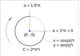
Many people think of a circle in “degrees”, where a circle is 360 degrees. However, most computer languages think in radians, where there are 2π radians in a circle. So if we sweep an angle, α from 0 (starting on the right) counter-clockwise through 2π, we end up in the same place, and have drawn a complete circle.
| Degrees | Radians |
|---|---|
| 0=360 | 0=2π |
| 90 | π/2 |
| 180 | π |
| 270 | 3π/2 |
As we perform the sweep, we use sin and cos to find the x and y coordinate corresponding to each angle. Understanding that this will give us a point relative to coordinate (0,0), we add an offset to the center of the circle.
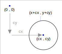
Therefore, given a radius of “r” and a center point (cx,cy), for any angle α:
- x = cx + r * cos(α)
- y = cy + r * sin(α)
The final puzzle piece is how much to increment α at each iteration, to ensure that every pixel is drawn properly?
C (Circumference of a circle) = π * d (diameter)
d = r (radius) * 2, therefore
C = 2πr
C is the number of pixels you have to draw, and a complete circle is 2π radians, so:
αi (incremental angle) = 2π / 2πr
And, what’s nice about radians is that everything cancels:
αi = 1 / r
In code, drawing a circle using trig would look like this:
const pi2=2*Math.PI;

function XtrigCircle(cx , cy , radius , r,g,b){
  var ai=1/radius; // incremental angle
  var x,y;

  for(var a = 0 ; a<pi2 ; a+=ai){
    x=Math.trunc( radius * Math.cos(a) );
    y=Math.trunc( radius * Math.sin(a) );

    plot( cx + x , cy + y ,r,g,b);
  }
}
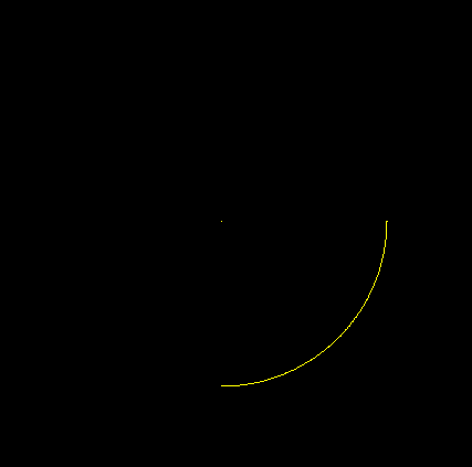
Here is a sample output using 0..π/2 (90 degrees) in order to demonstrate how the sweep works:
This works fine for an outline of a circle, but how do we draw a filled circle?
At first thought, drawing concentric circles (incrementing the radius) seems like a good idea, but it’s computationally-expensive.
Instead, we can exploit the symmetrical properties of a circle:
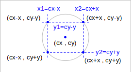
The concept is to do a 90-degree sweep through the (+,+) quadrant to get all of the (x,y) points, but use symmetry to mirror them within the other quadrants. Here is a revised circle-outline function using symmetry:
const piDiv2=Math.PI/2;

function XtrigCircle2( cx , cy , radius , r,g,b ){
  var ai=1/radius;
  var x,y;

  for( var a=0 ; a<=piDiv2 ; a+=ai ){
    x=Math.trunc( radius * Math.cos(a) );
    y=Math.trunc( radius * Math.sin(a) );

    plot( cx+x , cy+y , r,g,b ); // lower-right
    plot( cx-x , cy+y , r,g,b ); // lower-left
    plot( cx+x , cy-y , r,g,b ); // upper-right
    plot( cx-x , cy-y , r,g,b ); // upper-left
  }
}
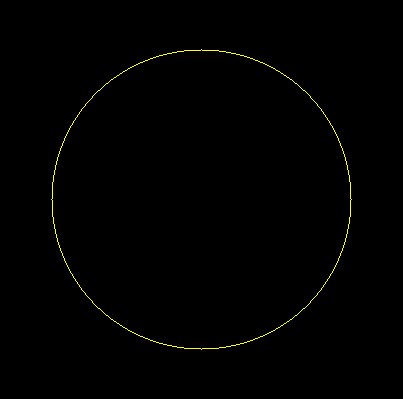
Output from the above:
To convert this to a filled circle, we loop from the left-half to the right-half:
function XtrigFillCircle( cx , cy , radius ,r,g,b ){
  var ai=1/radius;
  var x,y,x1,x2,y1,y2;

  for(var a=0 ; a<=piDiv2 ; a+=ai) {  // see above for piDiv2
    x=Math.trunc( radius * Math.cos(a) );
    y=Math.trunc( radius * Math.sin(a) );

    y1=cy-y;
    y2=cy+y;
    x1=cx-x;
    x2=cx+x;

    for(var xx=x1 ; xx<=x2 ; xx++){
      plot( xx , y1 , r,g,b );  // upper half
      plot( xx , y2 , r,g,b );  // lower half
    }
  }
}
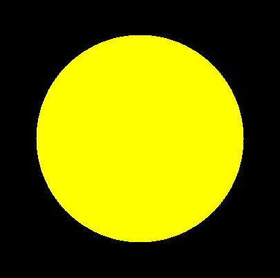
Here is the output of the trig-fill function:
Quadratic Circles
Aside from trigonometry, a circle can be defined by this quadratic equation:
x2 + y2 = r2
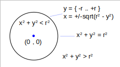
As you can see, this is related to the Pythagorean theorem, where any given radius of the circle is the hypotenuse of a right triangle (similar to trigonometry).
| x2 + y2 = r2 | (x,y) lies on the circumference |
| x2 + y2 < r2 | (x,y) lies on the interior |
| x2 + y2 > r2 | (x,y) lies outside |
Instead of sweeping a range of angles in order to draw the circumference, we can sweep a range of y values { -r .. r }, then for a given y, solve for x:
y = { -r .. r }
x = sqrt( r2 – y2 )
Taking in to account an offset to the center, we can plot the following coordinates:
- ( cx – x , cy + y ) // left half
- ( cx + x , cy + y ) // right half
Further, we can exploit symmetry, as we did above for the trig-based function by cutting the range in half, where y = { 0 .. r }
- (cx -x , cy -y ) // upper-left
- (cx+x , cy-y) // upper-right
- (cx-x , cy+y) // lower-left
- (cx+x , cy+y) //lower-right
Here is an example for drawing solid circles using the quadratic equation for a circle:
function XquadFillCircle( cx , cy , radius , r,g,b ){
  var x,xx,y,x1,x2,y1,y2;

  var ys, rs=radius * radius;

  for( y=0 ; y<=r ; y++ ){
    ys=y*y;
    x=Math.trunc( Math.sqrt( rs-ys ) );

    y1=cy-y;
    y2=cy+y;
    x1=cx-x;
    x2=cx+x;

    for( xx=x1 ; xx<=x2 ; xx++ ){
      plot( xx , y1 , r,g,b );  // top half
      plot( xx , y2 , r,g,b );  // bottom half
    }
  }
}
This produces nearly the same filled circle from the trig-fill example above:
However, if we do just an outline by plotting just x1 and x2 rather than looping, we get the following:
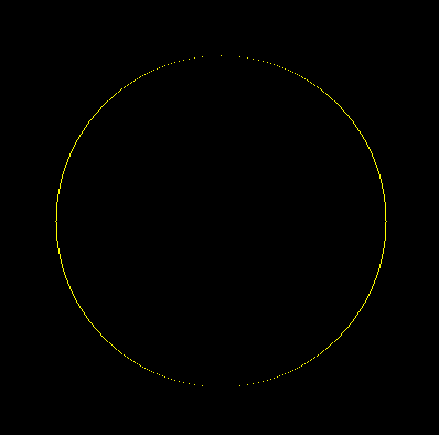
The gaps at the top and bottom occur because our code assumes there is only one x coord for every given y coord, and we are using y as our independent variable. As the slope increases beyond 45 degrees, we would need to use x as the independent variable in order to maintain single-pixel stepping.
To accomplish this we can exploit another symmetry of circles.
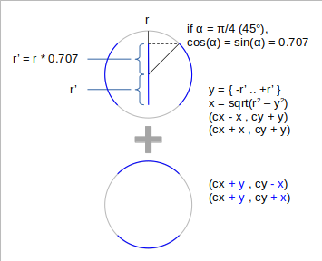
If an angle is below 45 degrees ( π//4 ) we can single-step y (top, partial circle in the diagram above). However, since x and y are symmetrical, we can swap them in order to form the top and bottom of the circle (bottom, partial circle in the diagram above).
The point where 45 degrees ( π//4 ) intercepts the vertical axis can be found by two different methods:
if α = π/2 then cos(α) = sin(α) = 0.707
and
if right Δ with hypotenuse r=1, and sides a=b, then
r2 = a2 + b2
Since a = b,
r2 = 2a2
Since r=1,
a2 = 1/2, and
a = 0.707
So, if we want to loop from our intercept point…
r’ = r * 0.707, and our range is
y = { 0 .. r’ }
In Javascript, it looks like this:
function XquadCircle( cx , cy , radius , r,g,b ){
  var x,y,x1,x2,y1,y2;
  var rs=radius*radius;
  var ys;
  var rp=Math.trunc( radius * 0.707 );

  for( y=0 ; y<=rp ; y++){
    ys=y*y;
    x=Math.trunc( Math.sqrt(rs - ys) );

    plot( cx-x , cy-y ,r,g,b );  // left-upper
    plot( cx+x , cy-y ,r,g,b );  // right-upper
    plot( cx-x , cy+y ,r,g,b );  // left-lower
    plot( cx+x , cy+y ,r,g,b );  // right-lower
  }
}
And, the output looks like this:
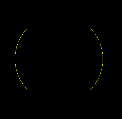
As expected, we see the left and right sides. To get the top and bottom, we need to add four more plots which transpose x and y offsets:
for(y...
  ...
  plot( cx-y , cy-x ,r,g,b );  // top-left
  plot( cx-y , cy+x ,r,g,b );  // bottom-left
  plot( cx+y , cy-x ,r,g,b );  // top-right
  plot( cx+y , cy+x ,r,g,b );  // bottom-right
  ...
}
And we get a complete circle:
Conclusion
Making circles using the quadratic formula for a circle is fast and easy, and way more computationally-efficient.